 ,
,

A Tutorial on Clustering Algorithms
Introduction | K-means | Fuzzy C-means | Hierarchical | Mixture of Gaussians | Links
Fuzzy
C-Means Clustering
The
Algorithm
Fuzzy c-means (FCM) is a method of clustering which allows one piece of data
to belong to two or more clusters. This method (developed by Dunn
in 1973 and improved by Bezdek in 1981) is frequently
used in pattern recognition. It is based on minimization of the following objective
function:
,
where m
is any real number greater than 1, uij is the degree of
membership of xi in the cluster j, xi
is the ith of d-dimensional measured data, cj is
the d-dimension center of the cluster, and ||*|| is any norm expressing the
similarity between any measured data and the center.
Fuzzy partitioning is carried
out through an iterative optimization of the objective function shown above,
with the update of membership uij and the cluster centers
cj by:
 ,
,

This iteration will
stop when  , where
  is a termination criterion between 0 and 1, whereas k are the iteration
steps. This procedure converges to a local minimum or a saddle point of Jm.
is a termination criterion between 0 and 1, whereas k are the iteration
steps. This procedure converges to a local minimum or a saddle point of Jm.
The algorithm is composed
of the following steps:
|
Remarks
As already told, data are
bound to each cluster by means of a Membership Function, which represents the
fuzzy behaviour of this algorithm. To do that, we simply have to build an appropriate
matrix named U whose factors are numbers between 0 and 1, and represent the
degree of membership between data and centers of clusters.
For a better understanding, we may consider this simple mono-dimensional example.
Given a certain data set, suppose to represent it as distributed on an axis.
The figure below shows this:

Looking at the picture, we may identify two clusters in proximity of the two data concentrations. We will refer to them using ‘A’ and ‘B’. In the first approach shown in this tutorial - the k-means algorithm - we associated each datum to a specific centroid; therefore, this membership function looked like this:
In the FCM approach, instead, the same given datum does not belong exclusively to a well defined cluster, but it can be placed in a middle way. In this case, the membership function follows a smoother line to indicate that every datum may belong to several clusters with different values of the membership coefficient.
In the figure above, the datum shown as a red marked spot belongs more to the B cluster rather than the A cluster. The value 0.2 of ‘m’ indicates the degree of membership to A for such datum. Now, instead of using a graphical representation, we introduce a matrix U whose factors are the ones taken from the membership functions:


(a) (b)
The number of rows
and columns depends on how many data and clusters we are considering. More exactly
we have C = 2 columns (C = 2 clusters) and N rows, where C is the total number
of clusters and N is the total number of data. The generic element is so indicated:
uij.
In the examples above we have considered the k-means (a) and FCM (b) cases.
We can notice that in the first case (a) the coefficients are always unitary.
It is so to indicate the fact that each datum can belong only to one cluster.
Other properties are shown below:


An
Example
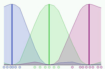
Here, we consider the simple case of a mono-dimensional application of the FCM.
Twenty data and three clusters are used to initialize the algorithm and to compute
the U matrix. Figures below (taken from our interactive
demo) show the membership value for each datum and for each cluster. The
color of the data is that of the nearest cluster according to the membership
function.
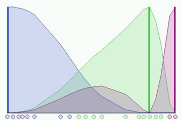
In the simulation
shown in the figure above we have used a fuzzyness coefficient m = 2 and we
have also imposed to terminate the algorithm when  .
The picture shows the initial condition where the fuzzy distribution depends
on the particular position of the clusters. No step is performed yet so that
clusters are not identified very well. Now we can run the algorithm until the
stop condition is verified. The figure below shows the final condition reached
at the 8th step with m=2 and =0.3:
.
The picture shows the initial condition where the fuzzy distribution depends
on the particular position of the clusters. No step is performed yet so that
clusters are not identified very well. Now we can run the algorithm until the
stop condition is verified. The figure below shows the final condition reached
at the 8th step with m=2 and =0.3:
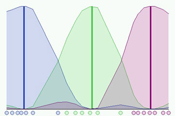
Is it possible to
do better? Certainly, we could use an higher accuracy but we would have also
to pay for a bigger computational effort. In the next figure we can see a better
result having used the same initial conditions and =0.01,
but we needed 37 steps!
It is also important to notice that different initializations cause different evolutions of the algorithm. In fact it could converge to the same result but probably with a different number of iteration steps.
Bibliography
Fuzzy C-means interactive demo