A Tutorial on Clustering Algorithms
Introduction | K-means | Fuzzy C-means | Hierarchical | Mixture of Gaussians | Links
Hierarchical
Clustering Algorithms
How
They Work
Given a set of N items to be clustered, and an N*N distance (or similarity)
matrix, the basic process of hierarchical clustering (defined by S.C.
Johnson in 1967) is this:
Step 3 can be done
in different ways, which is what distinguishes single-linkage from
complete-linkage and average-linkage clustering.
In single-linkage clustering (also called the connectedness
or minimum method), we consider the distance between one cluster and
another cluster to be equal to the shortest distance from any member
of one cluster to any member of the other cluster. If the data consist of similarities,
we consider the similarity between one cluster and another cluster to be equal
to the greatest similarity from any member of one cluster to any member
of the other cluster.
In complete-linkage clustering (also called the diameter or
maximum method), we consider the distance between one cluster and another
cluster to be equal to the greatest distance from any member of one cluster
to any member of the other cluster.
In average-linkage clustering, we consider the distance between one
cluster and another cluster to be equal to the average distance from
any member of one cluster to any member of the other cluster.
A variation on average-link clustering is the UCLUS method of R.
D'Andrade (1978) which uses the median distance, which is much more
outlier-proof than the average distance.
This kind of hierarchical clustering is called agglomerative because it merges clusters iteratively. There is also a divisive hierarchical clustering which does the reverse by starting with all objects in one cluster and subdividing them into smaller pieces. Divisive methods are not generally available, and rarely have been applied.
(*) Of course there is no point in having all the N items grouped in a single cluster but, once you have got the complete hierarchical tree, if you want k clusters you just have to cut the k-1 longest links.
Single-Linkage
Clustering: The Algorithm
Let’s now take a deeper look at how Johnson’s algorithm works in
the case of single-linkage clustering.
The algorithm is an agglomerative scheme that erases rows and columns in the
proximity matrix as old clusters are merged into new ones.
The N*N proximity matrix is D = [d(i,j)]. The clusterings are assigned sequence numbers 0,1,......, (n-1) and L(k) is the level of the kth clustering. A cluster with sequence number m is denoted (m) and the proximity between clusters (r) and (s) is denoted d [(r),(s)].
The algorithm is composed of the following steps:
|
An
Example
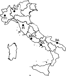
Let’s now see a simple example: a hierarchical clustering of distances
in kilometers between some Italian cities. The method used is single-linkage.
Input distance matrix (L = 0 for all the clusters):
BA |
FI |
MI |
NA |
RM |
TO |
|
BA |
0 |
662 |
877 |
255 |
412 |
996 |
FI |
662 |
0 |
295 |
468 |
268 |
400 |
MI |
877 |
295 |
0 |
754 |
564 |
138 |
NA |
255 |
468 |
754 |
0 |
219 |
869 |
RM |
412 |
268 |
564 |
219 |
0 |
669 |
TO |
996 |
400 |
138 |
869 |
669 |
0 |

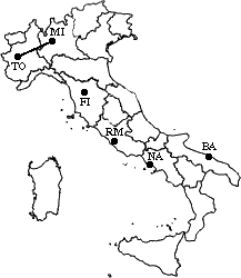
The nearest pair
of cities is MI and TO, at distance 138. These are merged into a single cluster
called "MI/TO". The level of the new cluster is L(MI/TO) = 138 and
the new sequence number is m = 1.
Then we compute the distance
from this new compound object to all other objects. In single link clustering
the rule is that the distance from the compound object to another object is
equal to the shortest distance from any member of the cluster to the outside
object. So the distance from "MI/TO" to RM is chosen to be 564, which
is the distance from MI to RM, and so on.
After merging MI with TO we obtain the following matrix:
BA |
FI |
MI/TO |
NA |
RM |
|
BA |
0 |
662 |
877 |
255 |
412 |
FI |
662 |
0 |
295 |
468 |
268 |
MI/TO |
877 |
295 |
0 |
754 |
564 |
NA |
255 |
468 |
754 |
0 |
219 |
RM |
412 |
268 |
564 |
219 |
0 |
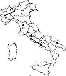
min d(i,j) = d(NA,RM)
= 219 => merge NA and RM into a new cluster called NA/RM
L(NA/RM) = 219
m = 2
BA |
FI |
MI/TO |
NA/RM |
|
BA |
0 |
662 |
877 |
255 |
FI |
662 |
0 |
295 |
268 |
MI/TO |
877 |
295 |
0 |
564 |
NA/RM |
255 |
268 |
564 |
0 |
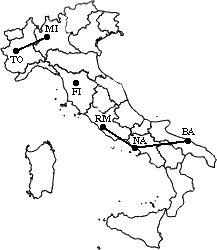
min d(i,j) = d(BA,NA/RM) = 255 =>
merge BA and NA/RM into a new cluster called BA/NA/RM
L(BA/NA/RM) = 255
m = 3
BA/NA/RM |
FI |
MI/TO |
|
BA/NA/RM |
0 |
268 |
564 |
FI |
268 |
0 |
295 |
MI/TO |
564 |
295 |
0 |
min d(i,j) = d(BA/NA/RM,FI) = 268
=> merge BA/NA/RM and FI into a new cluster called BA/FI/NA/RM
L(BA/FI/NA/RM) = 268
m = 4
BA/FI/NA/RM |
MI/TO |
|
BA/FI/NA/RM |
0 |
295 |
MI/TO |
295 |
0 |
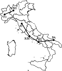
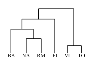
Finally, we merge the last two clusters at level 295.
The process is summarized by the following hierarchical tree:
Problems
The main weaknesses of agglomerative clustering methods are:
Bibliography
Hierarchical clustering interactive demo